
Due to the many international requests I received – this is a translation of my original blog post.
You can even download the Excel file I used for creating this blog post here.
Many of us know and like the MATCH()- function in Microsoft Excel.
It offers the possibility to locate the position of an element (not its value!) in an array resp. a matrix according to the search criteria.
Unfortunately, this very helpful functionality has an issue since – although Excel normally indicates an „array“ as an area consisting of multiple rows or multiple columns – for the function MATCH() Excel principally only accepts an area consisting of a single row or a single column.
[bctt tweet=“Excel only accepts an area consisting of a single column or a single row when using the function #MATCH().“ username=“hdcnews“]
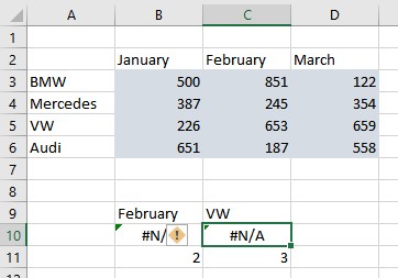
Screenshot #1 – Value view
This is an issue if you select an array of multiple rows or columns (in our sample the complete table A2:D6).
Let’s have a look at the formula view:
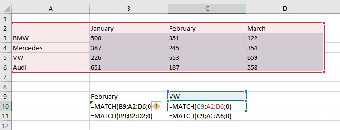
Screenshot #2 – formula view
In our sample we defined in cell C10 (currently marked green) the array for the MATCH()-function- for the complete data table (A2:D6, marked red).
But, as we can see in our upper screenshot #1, this leads to an #N/A error.
In the cell below we defined the array for the MATCH()-function on a single column area (here: A3:A6).
If we have a look at the result (see screenshot #1), we ‚ll see it finally delivers the correct result.
Of course this is not working with an array consisting of several rows – t always has to be a single row.
Unfortunately, this aspect isn’t mentioned in Excel – neither in the functions dialog nor in the help.
So, if you ever have an issue with the MATCH()-function, first check, if your matrix/array really consists of just a single column or a single row.
Special usage of MATCH()
But how can we use this ingenious function to find an element in a table which fits to several conditions?
As a sample let’s use the following table, while the task is as follows:
Find the price for the product which consists of „flour“, is of type “550” and which has a weight of “500g”.

You got the solution?
A tiny hint:
Without an additional function we won’t get along, right?
VLOOKUP() doesn’t really help us, since VLOOKUP() only checks the first column of an array.
Admitted, it would be pretty easy to filter and select the table and using the partial result of the filtered table for further calculations.
But, what if we want to show the complete table above (for some reason)?
Solution
We additionally use the INDEX()-function of Microsoft Excel in combination with the MATCH()-function.
To make it easier to read and understand we name the value area of the table (A2:D10, marked blue) as “flourprices”.
Furthermore we enter „flour“ in cell A13, since we want to search for this expression.
In cell B13 we enter “550” – this is the type of flour we look for and in cell C3 we enter “500” – the weight we are looking for.
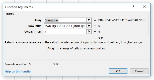
In the green cell (D13) we finally enter the following formula:
=INDEX(flourprices;MATCH(A13&B13&C13;INDEX(flourprices;;1)&INDEX(flourprices;;2)&INDEX(flourprices;;3);0);4)
IMPORTANT:
In this case we need the array formula – and not as usual the standard formula.
To let Excel know to use the array formula, we finish our entry by using the keystroke combo <Ctrl> + <Shift> + <Enter> – instead of normally just <Enter>.
Afterwards our formula looks like this:
{=INDEX(flourprices;MATCH(A13&B13&C13;INDEX(flourprices;;1)&INDEX(flourprices;;2)&INDEX(flourprices;;3);0);4)}
So, the final function now has additional curly brackets (marked red).
What did we do and why does Excel deliver the correct result?
OK, we now know MATCH() only searches in single rows or single columns – but our data table (here: flourprices) has multiple rows and columns.
On the other hand, the array version of INDEX() delivers an element in a multi-column and multi-row(!) array.
Unfortunately, it doesn’t help to find the element itself, but rather delivers the value of the element we defined in the array using rows and columns.
Therefore, we simply combine both functions.
We enter the value area of the table we defined before – in this case „flourprices”.
But before we have a look at the „Row_num“-argument (this will be a bit longer), I want to explain the „Column_num“-argument.
For the column (third argument) we enter “4” since we want to have the price of the product and this is located in the 4. column of our value range.
Now, we get to the „Row_num“-argument of the INDEX-function (the second field in the dialog box) and heer we use a “trick”:
Instead of entering a fixed cell, we keep it variable and use the MATCH()-function.
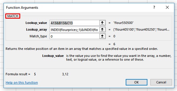
As the search criteria for the MATCH()-function we enter a combination, while we concatenate each search criteria with an ampersand – commonly known as „&“.
So, we enter A13&B13&C13 – there, our criteria are located Excel is supposed to look for in our value range.
Everything fine so far?
Now, we only have to „explain“ Excel, where to find the values – so, in which columns (this can be very important, if we use a table consisting of identical values in different columns).
We now need again the INDEX()-function:
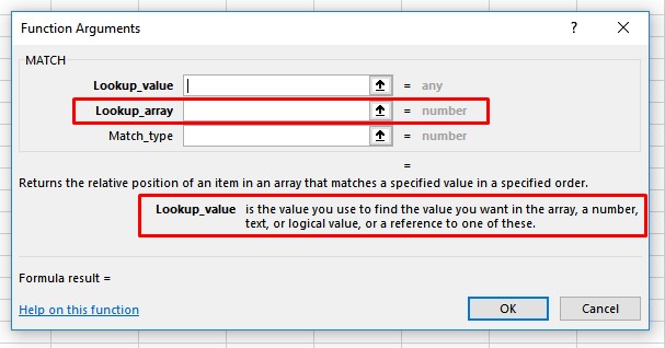
For the argument in the “Lookup_array” of the MATCH()-function (see screenshot above) we first enter the column, where Excel should search for the value of A13.
This is the column A – but we don’t want to select just the area (here: A2:A10), but rather re-use our nice name range “flourprices”.
Therefore, we use the INDEX()-function and tell it to use the first column of our name range “flourprices”:
INDEX(flourprices;;1)
We don’t need the row in this INDEX()-function since we want to get the whole column, to let Excel search in it with MATCH() using “flour”.
To ensure, Excel also searches simultaneously(!) for our entry in cell B13 (this is the type of flour), we add to the first INDEX()-function a second one by using an ampersand “&” – just like we did in the „Lookup_value“.
But this time we tell Excel, it’s supposed to search for the flour prices in column 2:
INDEX(flourprices;;1)&INDEX(flourprices;;2)
Finally, we need to define the third column, since we also need to search for the weight (we entered this criteria in cell C13).
INDEX(flourprices;;1)&INDEX(flourprices;;2)&INDEX(flourprices;;3)
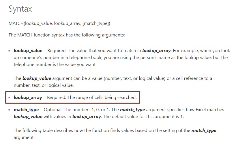
Now, we only have to define the argument “Match_type” for MATCH() (see screenshot above) by entering the value „0“ (3. argument), since we want to have an exact match.
That’s it ;)
I hope you have great fun using Excel and best wishes
Eric
One Reply to “Matrix issue using MATCH()”